
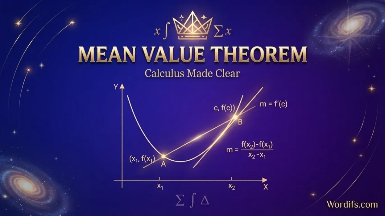
The Mean Value Theorem (MVT) is an important result in calculus that connects a function’s average rate of change over an interval with its instantaneous rate of change at a particular point. In simple terms, it guarantees that, under certain conditions, a function has at least one point where its tangent line has the same slope as the secant line connecting the interval’s endpoints.
The Mean Value Theorem is widely used in differential calculus, graph analysis, optimization, and mathematical proofs. It helps explain how derivatives describe the behavior of functions and provides a foundation for other important results, including the relationship between increasing functions and positive derivatives. Understanding its formula, conditions, and worked examples makes it much easier to apply in calculus problems.
Quick Answer: What Is the Mean Value Theorem?
The Mean Value Theorem states that if a function (f(x)) is continuous on a closed interval ([a,b]) and differentiable on the open interval ((a,b)), then there is at least one number (c) between (a) and (b) such that
[
f'(c)=\frac{f(b)-f(a)}{b-a}.
]
This means the instantaneous rate of change at some interior point equals the average rate of change over the entire interval.
What Is the Mean Value Theorem in Calculus?
The Mean Value Theorem is a fundamental theorem of differential calculus. It establishes a connection between the derivative of a function at a specific point and the function’s overall change across an interval.
To understand the idea, imagine driving 120 miles in two hours. Your average speed is 60 miles per hour. If your speed changes continuously during the trip, then at some moment your instantaneous speed must have been exactly 60 miles per hour.
This is an intuitive illustration of the Mean Value Theorem. The theorem does not say that your speed stays constant. It guarantees that, under the appropriate continuity and differentiability conditions, the instantaneous rate equals the average rate at least once.
In mathematics, the theorem applies to functions that satisfy two conditions:
- The function must be continuous on the closed interval from (a) to (b).
- The function must be differentiable on the open interval between (a) and (b).
When these conditions hold, at least one suitable point (c) exists between the endpoints.
What Does the Mean Value Theorem Mean in Simple Words?
In simple words, the Mean Value Theorem says that a function’s average change over an interval must match its instantaneous change at least once somewhere inside that interval.
For a graph, imagine drawing a straight line between two points on the curve. This line is called a secant line. The Mean Value Theorem guarantees that at some interior point, the curve has a tangent line parallel to that secant line.
The slopes are equal because both lines represent the same rate of change.
Mean Value Theorem Formula
The standard Mean Value Theorem formula is
[
\boxed{f'(c)=\frac{f(b)-f(a)}{b-a}}
]
where (a<b) and (c\in(a,b)).
Each symbol has a specific meaning:
- (f(a)): The function’s value at the left endpoint.
- (f(b)): The function’s value at the right endpoint.
- (f'(c)): The derivative at the interior point (c).
- (\frac{f(b)-f(a)}{b-a}): The average rate of change over the interval.
- (c): A point strictly between (a) and (b) where the required equality holds.
The expression on the right is the slope of the secant line. The expression on the left is the slope of the tangent line.
Average Rate of Change vs. Instantaneous Rate of Change
The Mean Value Theorem connects two important calculus concepts.
Average rate of change measures how much a function changes between two points:
[
\frac{f(b)-f(a)}{b-a}.
]
Instantaneous rate of change measures how quickly the function changes at one particular point. It is represented by the derivative (f'(c)).
The theorem guarantees that these two rates are equal at least once inside the interval when its assumptions are satisfied.
Conditions of the Mean Value Theorem
Before applying the Mean Value Theorem, you must verify that the function meets both required conditions. If either condition fails, the theorem cannot be applied directly to that interval.
1. Continuity on the Closed Interval
The function must be continuous on ([a,b]), including both endpoints.
A continuous function has no breaks, jumps, or holes within the interval. You should be able to draw its graph over the interval without lifting your pencil.
For example, polynomial functions such as (f(x)=x^2+3x) are continuous everywhere, so they satisfy this condition on any closed interval.
However, a function with a jump discontinuity inside the interval does not satisfy the continuity requirement.
2. Differentiability on the Open Interval
The function must be differentiable at every point in ((a,b)).
Differentiability means the derivative exists at each interior point. A sharp corner, cusp, or vertical tangent may prevent a function from being differentiable at a particular point.
For example, (f(x)=|x|) is continuous everywhere but is not differentiable at (x=0). Therefore, the Mean Value Theorem cannot be applied to an interval that contains zero in its interior.
Mean Value Theorem Conditions at a Glance
| Condition | Required interval | What to check |
| Continuity | Closed interval ([a,b]) | No discontinuities, including at endpoints |
| Differentiability | Open interval ((a,b)) | Derivative exists at every interior point |
| Conclusion | Interior point (c) | At least one point satisfies the MVT equation |
Always check both conditions before calculating the value of (c).
Mean Value Theorem Examples With Step-by-Step Solutions
Worked examples are one of the best ways to understand how the theorem is used in calculus.
Example 1: Apply the Mean Value Theorem to (f(x)=x^2)
Problem: Find the value of (c) guaranteed by the Mean Value Theorem for
[
f(x)=x^2,\qquad [1,3].
]
Step 1: Check the conditions.
Since (f(x)=x^2) is a polynomial, it is continuous and differentiable everywhere. Therefore, both conditions are satisfied on ([1,3]).
Step 2: Calculate the average rate of change.
The endpoint values are
[
f(1)=1,\qquad f(3)=9.
]
Using the formula,
[
\frac{f(3)-f(1)}{3-1}
=\frac{9-1}{2}=4.
]
Step 3: Find the derivative.
Differentiate the function:
[
f'(x)=2x.
]
Step 4: Set the derivative equal to the average rate.
[
2c=4.
]
Solving gives
[
\boxed{c=2}.
]
Because (2) lies between (1) and (3), the answer satisfies the theorem.
Final answer: (c=2).
Example 2: Apply the Theorem to a Cubic Function
Problem: Find the value of (c) for
[
f(x)=x^3,\qquad [1,2].
]
Step 1: Verify continuity and differentiability.
The function is a polynomial, so it meets both conditions.
Step 2: Calculate the secant slope.
[
f(1)=1,\qquad f(2)=8.
]
Therefore,
[
\frac{f(2)-f(1)}{2-1}
=\frac{8-1}{1}=7.
]
Step 3: Find the derivative.
[
f'(x)=3x^2.
]
Step 4: Solve for (c).
Set the derivative equal to the secant slope:
[
3c^2=7.
]
Thus,
[
c^2=\frac73
]
and
[
c=\pm\sqrt{\frac73}.
]
Since (c) must lie in the open interval ((1,2)), only the positive solution is valid:
[
\boxed{c=\sqrt{\frac73}}.
]
The negative solution is outside the interval and must be rejected.
Example 3: Find (c) for a Linear Function
Problem: Apply the Mean Value Theorem to
[
f(x)=5x-2,\qquad [0,4].
]
Step 1: Check the conditions.
A linear function is continuous and differentiable everywhere.
Step 2: Calculate the average rate of change.
[
f(0)=-2,\qquad f(4)=18.
]
Therefore,
[
\frac{18-(-2)}{4-0}=\frac{20}{4}=5.
]
Step 3: Differentiate.
[
f'(x)=5.
]
The derivative equals the average rate of change at every point.
Consequently, every value of (c) in ((0,4)) satisfies the Mean Value Theorem.
Final answer: Any (c\in(0,4)).
This example shows that the theorem guarantees at least one point, not necessarily exactly one point.
How to Solve Mean Value Theorem Problems
You can use the following method for most standard Mean Value Theorem exercises.
<box gap={2}> <row align=start gap={3}> <box background=”surface-secondary” radius=”lg” size=”40px” align=center justify=center> <title size=”lg”>1</title> </box> <box flex=”1″ gap={1}> **Identify the function and interval.**
Write down f(x), the left endpoint a, and the right endpoint b.
</box>
</row> <row align=start gap={3}> <box background=”surface-secondary” radius=”lg” size=”40px” align=center justify=center> <title size=”lg”>2</title> </box> <box flex=”1″ gap={1}> **Verify both conditions.**
Confirm continuity on [a,b] and differentiability on (a,b).
</box>
</row> <row align=start gap={3}> <box background=”surface-secondary” radius=”lg” size=”40px” align=center justify=center> <title size=”lg”>3</title> </box> <box flex=”1″ gap={1}> **Calculate the average slope.**
Evaluate the function at both endpoints and calculate f(b)-f(a)b-a.
</box>
</row> <row align=start gap={3}> <box background=”surface-secondary” radius=”lg” size=”40px” align=center justify=center> <title size=”lg”>4</title> </box> <box flex=”1″ gap={1}> **Differentiate the function.**
Find f'(x) using the appropriate differentiation rules.
</box>
</row> <row align=start gap={3}> <box background=”surface-secondary” radius=”lg” size=”40px” align=center justify=center> <title size=”lg”>5</title> </box> <box flex=”1″ gap={1}> **Solve and check the interval.**
Set the derivative equal to the average slope, solve for c, and keep only solutions inside (a,b).
</box>
</row> </box>
Following these steps makes your solution easier to understand and helps prevent algebraic mistakes.
Mean Value Theorem vs. Rolle’s Theorem
Rolle’s Theorem is a special case of the Mean Value Theorem.
Both theorems require a function to be continuous on a closed interval and differentiable on its interior. However, Rolle’s Theorem adds the condition that the endpoint values are equal:
[
f(a)=f(b).
]
Under these conditions, Rolle’s Theorem guarantees at least one point (c\in(a,b)) where
[
f'(c)=0.
]
The Mean Value Theorem does not require equal endpoint values. Instead, it requires the derivative to equal the average slope between the endpoints.
| Feature | Mean Value Theorem | Rolle’s Theorem |
| Continuity on ([a,b]) | Required | Required |
| Differentiability on ((a,b)) | Required | Required |
| Equal endpoint values | Not required | Required |
| Guaranteed derivative | (f'(c)=\frac{f(b)-f(a)}{b-a}) | (f'(c)=0) |
| Geometric meaning | Parallel tangent and secant lines | Horizontal tangent line |
When (f(a)=f(b)), the secant slope is zero, so the Mean Value Theorem produces the same conclusion as Rolle’s Theorem.
Applications of the Mean Value Theorem
The Mean Value Theorem is more than a formula for solving textbook problems. It is also a useful tool for understanding and proving properties of functions.
1. Understanding Rates of Change
The theorem connects average and instantaneous rates of change.
In physics, for example, the average velocity over a time interval is the total displacement divided by elapsed time. Under suitable differentiability conditions, the theorem guarantees a moment when instantaneous velocity equals that average velocity.
2. Proving a Function Is Increasing or Decreasing
The Mean Value Theorem can establish whether a function increases or decreases over an interval.
If (f'(x)>0) throughout an interval, the function is strictly increasing there. If (f'(x)<0) throughout an interval, the function is strictly decreasing.
To see why, take any two points (a<b). The theorem gives a point (c) between them such that
[
f(b)-f(a)=f'(c)(b-a).
]
Since (b-a>0), a positive derivative makes (f(b)-f(a)>0), confirming that the function increases.
3. Establishing Bounds on Function Values
Suppose (|f'(x)|\leq M) throughout an interval. The Mean Value Theorem implies that
[
|f(b)-f(a)|\leq M|b-a|.
]
This inequality shows that a bound on the derivative limits how quickly the function’s values can change.
Such bounds are useful in numerical analysis, error estimates, and mathematical proofs.
4. Comparing Two Functions
The theorem can also help compare function values by applying derivative information to their difference.
For example, if two differentiable functions have the same value at one point and their derivatives satisfy an appropriate inequality throughout an interval, the Mean Value Theorem can help establish an ordering between their values elsewhere.
This technique is useful in calculus proofs and mathematical analysis.
Common Mistakes to Avoid
When applying the Mean Value Theorem, watch for these common errors:
- Skipping the conditions: Do not assume the theorem applies just because you can calculate a derivative.
- Using the wrong interval: Continuity is required on the closed interval, while differentiability is required on the open interval.
- Reversing the average slope: Use (f(b)-f(a)) in the numerator and (b-a) in the denominator.
- Forgetting to differentiate: The equation must use (f'(c)), not the original function (f(c)).
- Accepting solutions outside the interval: Every valid (c) must satisfy (a<c<b).
- Assuming there is only one answer: The theorem guarantees at least one valid point, but there may be several or infinitely many.
Checking these details before submitting your answer can improve both accuracy and mathematical reasoning.
Frequently Asked Questions
1. What is the Mean Value Theorem in simple terms?
The Mean Value Theorem says that a continuous and differentiable function has at least one point where its instantaneous rate of change equals its average rate of change over a given interval.
2. What is the formula for the Mean Value Theorem?
The formula is
[
f'(c)=\frac{f(b)-f(a)}{b-a},
]
where (c) is between (a) and (b). The function must be continuous on ([a,b]) and differentiable on ((a,b)).
3. Why is the Mean Value Theorem important?
It connects derivatives with overall changes in function values. It is useful for analyzing rates of change, proving inequalities, studying increasing and decreasing functions, and establishing bounds on errors.
4. What are the two conditions of the Mean Value Theorem?
The function must be continuous throughout the closed interval ([a,b]) and differentiable throughout the open interval ((a,b)). Both conditions are necessary to apply the theorem as stated.
5. What is the difference between the Mean Value Theorem and Rolle’s Theorem?
The Mean Value Theorem guarantees a point where the derivative equals the average slope across the interval. Rolle’s Theorem requires equal endpoint values and guarantees a point where the derivative is zero.
6. Can the Mean Value Theorem have more than one solution?
Yes. The theorem guarantees at least one valid value of (c), but multiple values may satisfy the equation. For a linear function, every interior point may satisfy it.
7. Does the Mean Value Theorem apply to every function?
No. A function must satisfy the continuity and differentiability conditions on the specified interval. A discontinuity or a point where the derivative does not exist inside the interval prevents direct application of the theorem.
Final Thoughts
The Mean Value Theorem is a fundamental concept in calculus that connects the average rate of change of a function with its instantaneous rate of change. Its formula, (f'(c)=\frac{f(b)-f(a)}{b-a}), provides a systematic way to find points where these rates match.
To solve problems correctly, first verify continuity and differentiability, calculate the average slope, find the derivative, and solve for a point inside the interval. Understanding these steps also helps you apply the theorem to Rolle’s Theorem, function behavior, mathematical inequalities, and real-world rate-of-change problems.

Kalven Driost works on the Wordifs site producing reliable content while communicating through wordifs@gmail.com to support research editing publishing consistency transparency and audience focused knowledge sharing practices for modern readers.